Change … in general

With my recent move to the University of Alabama from the University of Florida, I starting thinking about the topic of change. In the context of quantitative investing, I started thinking about changes in basic rules that we take for given when investing quantitatively and what we can do about them.

Here’s an example – academics have long taught the CAPM, a model that predicts that companies with higher systematic risk (risk stemming from overall market conditions) should outperform companies with lower systematic risk. This makes intuitive sense… riskier companies, especially companies with higher risk exposure to overall economic conditions *should* give higher returns, on average. The empirical evidence in the 70s and 80s (in hindsight) was mixed, but in general we accepted this wisdom.

However, starting in the 1990s, we started to question this basic assumption. Fama French 1992, Table II documented this:

betaret

Companies are sorted by “pre-ranking betas” (simply the beta estimated using data from before the period we measure the returns) and the average monthly returns for the next year, by pre-beta deciles are presented. 1A and 1B are the 0-5% and 5-10% comapnies by pre-rnaking beta, 2-9 are the 2nd through 9th decile by pre-ranking beta, 10A and 10B are the 90-95% and 95-100% of firms by preranking beta.

Fama and French wrote, “the beta-sorted portfolios do not support the [CAPM]. … There is no obvious relation between beta and average returns.” [disclaimer: to my eyes, if I squint hard enough, I can sort of see a slight increase in average returns with beta, but the magnitude and monotonicity of the effect are both questionable.]

And so the decline of empirical belief in the CAPM started, and today, there is little faith that stocks with high market betas will outperform the market (although the CAPM is still widely taught). (see, for example “Is Beta Dead” from the Appendix of a popular Finance Textbook. )

In fact, the academic literature has made something of a 180 on this topic. The new hot anomaly is “low vol,” or “low beta.” This literature around this anomaly shows that the low volatility/low beta stocks actually outperform high volatility/high beta stocks and proposes several stories as to why this might be the case. If something so firmly grounded in theory can experience so complete a change, I think it’s a cautionary tale for *all* quantitative strategies … all things (including both the CAPM Beta and my time at Florida), run their course eventually.


Momentum Across Anomalies

In a new academic piece, we examine whether anomalies themselves exhibit momentum. Momentum in the context of investing refers to the idea that stocks that have done well recently continue to do well and stocks that have done poorly recently continue to do poorly. The momentum anomaly in stocks was widely publicized by Jagadeesh and Titman in their 1993 paper titled, “Returns to Buying Winners and Selling Losers: Implications for Stock Market Efficiency.”

We find this same idea holds for anomalies themselves. Examining 13 anomalies, we find anomalies that have performed well recently (in the last month), continue to do well next month. Anomalies that have been performing poorly recently continue to experience poor performance going forward. A chart makes this clear:

anomom

The chart documents the evolution of $10,000 invested in one of three strategies. The top line is a strategy that invests each month in the top half of the 13 anomalies (7 since investing in 6½ anomalies is hard) being analyzed, based on the 13 anomalies’ performance in the previous month. So, for example, if the value, momentum, size, profitability, accruals, investment level, and O-score anomalies did better than the other 6 anomalies we analyzed\ last month, the strategy would equally invest in these 7 anomalies. The bottom line does the opposite, investing in the bottom 6 anomalies and the middle line equally invests in all 13 anomalies across the entire period.

From the chart, it is clear that anomalies themselves exhibit momentum and the result is robust to the usual battery of academic tests. From a practitioner’s perspective, the implication is clear: if you’re interested in smart beta type investing, pick a strategy (or strategies) that has been doing well recently. From an academic’s perspective, the more interesting question is why. If you’re interested in our take on reasons for this, you can read our paper for some reasons we think we observe this momentum across anomalies.


Why invest quantitatively?

My current academic research currently focuses on personal characteristics of investors (specifically hedge fund managers) and how these characteristics affect their investments. For example, my paper on hedge fund managers’ marriages and divorecs shows that fund performance suffers during both marriages and divorces and argues this is a results of manager distraction from personal events. Another paper on hedge fund managers’ cars shows that fund managers who drive performance cars take more risks, without yielding additional returns.

This general agenda has led me to the firm belief that investors are swayed by behavioral biases in their investments. These biases can be the result of some intrinsic characteristic (such as a desire for sensation seeking, which leads to a preference for fast cars and risk in investments) or some time varying affect (such as a distraction from a major life event). Either way, these biases are hazardous to investment performance.

Quantitative investing gives an easy out to these biases. If we follow a fixed set of rules  when investing (and are faithful in following them), there’s no room for behavioral biases to creep in. A computer, relying on objective data from the markets, tells us what to buy and sell when. Getting married? No problem – just let the computer tell you what to do. Getting divorced? Same deal. Inherently a risk taker? There’s no scope for your gambling ways to affect your investing. Risk averse to the extreme? Again… no way for your timidity to stymie your investing.

This is one of the big advantages of quantitative investing.

Long short strategies at a time when we are at all time highs

Markets are at all time highs – this is not uncommon – markets (since they are supposed to go up) should be at, or near, all time highs much of the time. That doesn’t mean that investors cannot be nervous about this condition. A number of respected investors will encourage caution, citing “all-time highs” as a reason for caution. The worry, of course, is that the market will come crashing down.

spy

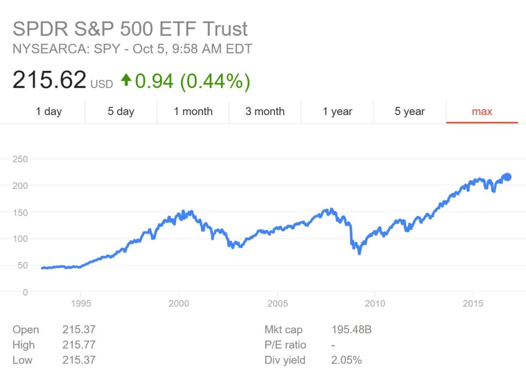
(SPY at all time highs right now!)

Long short strategies, which have both long, and short positions are a nice way to hedge against the potential of a large market downturn. When engaging in a long short strategy, the first decision to make is are you going to be completely hedged (that is, your long positions and short positions are roughly equal, in terms of market sensitivity), or are you going to have a long or short bias. This is ultimately a decision that resolves into the question, “can you time the market?” There are many perspectives on this, but my take is that this is hard to do and I am not going to focus on this.

Rather, I will focus on a question that arises once you have decided on a net exposure: what should you be long? and what should you be short? Some solutions include:

1. Going long and short completely separate strategies – for example, profitability for a long strategy and some short screen for a short. This has the advantage in that you are, at least in back tests, gaining on both ends. However, we know nothing about the correlations of the long and short legs and there may be situations in which we lose money on both ends if the long leg goes down and the short leg goes up!

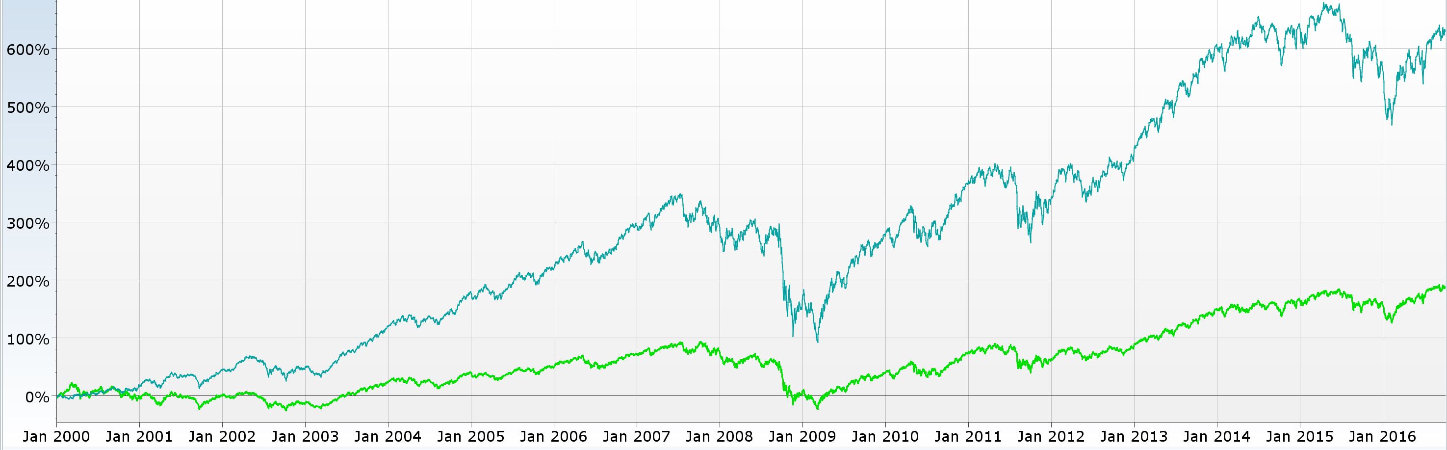
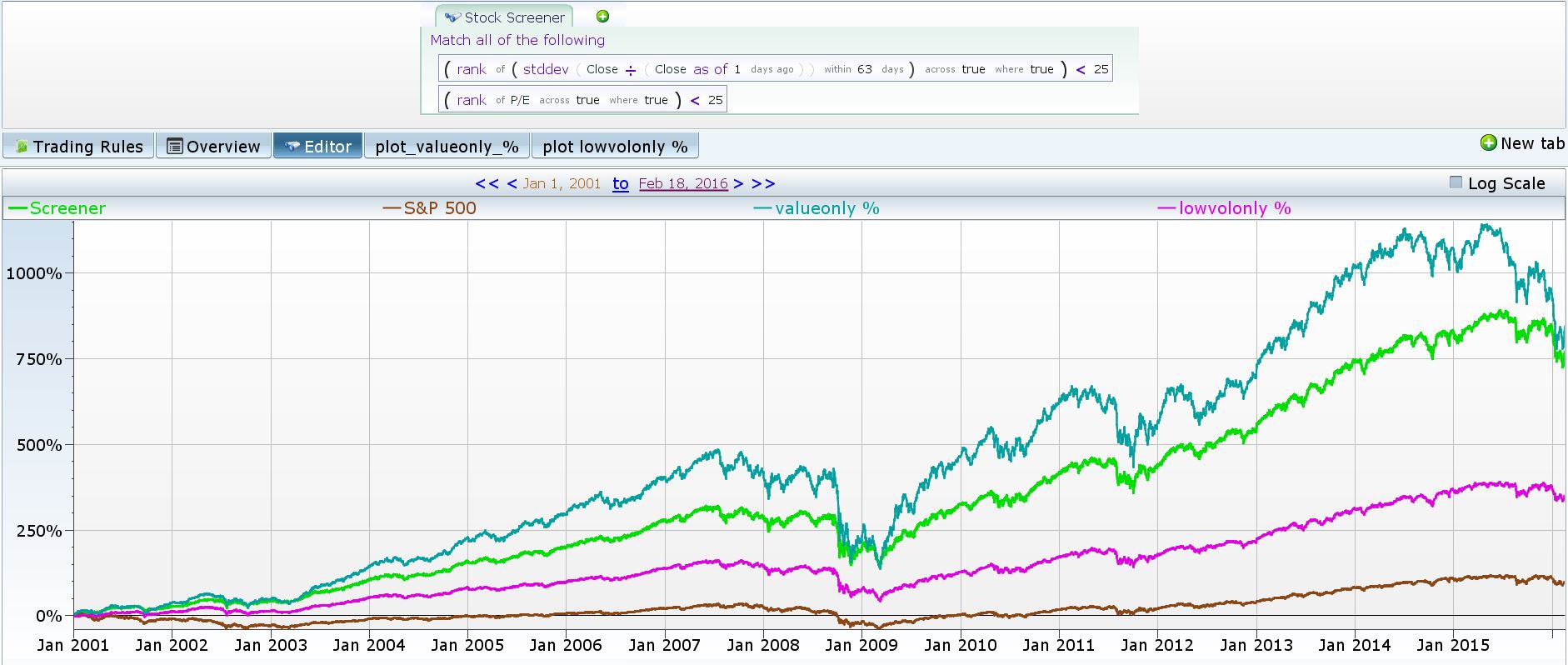
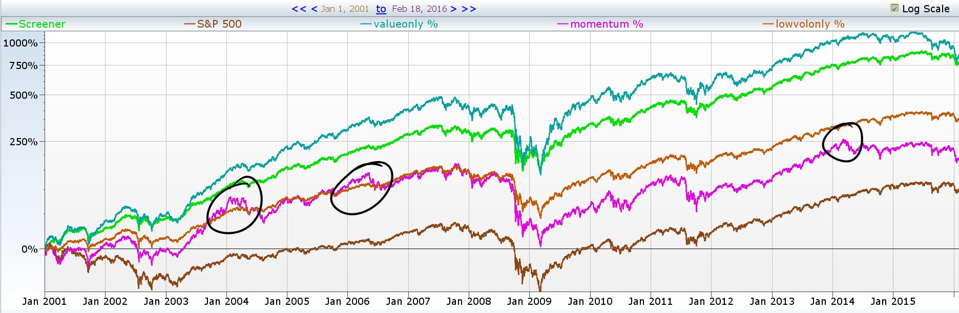
2. Going long and short separate ends of a single spectrum. For example, if we are separating stocks in the universe based on the PE measures, perhaps we go long low PE stocks (value stocks) and short high PE stocks (growth stocks).

vg


(Value – top line, growth, bottom line – we would make the difference in a long short strategy)

This has some advantages over the first technique, in that the stocks are otherwise likely to be similar in long and short legs, and hence the correlations should be high – thus the hedge from the short leg should work better. Also, this is the standard way in which academics document characteristics of stocks that affect future returns –  so there is a lot of literature and data easily available under this framework.

3. Going long something that’s “good” and being short the market. This is the most common way industry practitioners seem to run long short portfolios. Their long legs are driven by their proprietary research and secret signals but on the short side, they simply use the market. The real advantage to this is that from a practitioners perspective, shorting the market is much, much easier than shorting a collection of stocks. There is infinite liquidity in market indices and you never have to be worried about getting a locate.

These are just three possible ways to implement a long short strategy. Each with its own advantages and disadvantages. They are definitely psychologically useful when investing in markets that are at “all time highs,” but there’s no reason to restrict their use to such situations – they can be used any time you want to a hedge against potential large downturns in the markets.


The sky is falling … [but I’m not short]

With the Dow and other indices at record levels, there is no shortage of pundits out there warning of an impending correction, or worse. See, for example, http://money.cnn.com/2016/04/15/investing/stock-market-donald-trump-ted-cruz/ and http://thesovereigninvestor.com/exclusives/80-stock-market-crash-to-strike-in-2016/ .

Some of the fear mongers, unfortunately, have an ulterior motive for predicting doom and gloom. A number of advisers look at such predictions as free options – if there is a crash, they can sagely point to their warnings and say, “See, I called it.” Some can even monetize their call… raising funds as investors look to re-allocate their decimated portfolios to stem the bleeding. If there is no crash, well, no one will look back and call them out on their incorrect call.

To me, the real question is whether these prognosticators have their money where their mouth is. If they think a major crash is coming, are they short? Or at least in cash? If not, I find their warnings have little credibility. They might be right, they might be wrong – either way, they’re not betting their own money on the call.

As the famous saying from Paul Samuelson goes, Economists (using technical indicators), “predicted nine of the last five recessions.” It wouldn’t surprise me if unscrupulous financial advisers and nay-saying pundits predicted ninety.

Blending factors…. the problem with intersections

I have recently been working on an academic paper on using multiple factors to invest. This is a marked departure from most of my other academic work (which generally involves hedge fund data). This research is also directly relevant to my investing work. While the research itself is still ongoing and I am not ready to share the conclusions, I had a couple of insights on how difficult it is to combine factors that I’d share.

The technique I’ve been using to combine factors is looking for intersections – I believe value stocks outperform growth stocks and past winners outperform losers. I want to buy stocks that are both value stocks AND past winners. (Incidentally, there is a rigorous academic paper arguing for this exact factor combination by the managers of one of the most successful quantitative investing shops).

This works well… to an extent. The more factors you add, the fewer stocks will get through. As an example, if you wanted the top 10% of stocks by value (say P/E ratios) and the top 10% of stocks by past returns, and the two were uncorrelated, your filter would return about 1% of stocks in the universe. Adding a 3rd uncorrelated factor, say size (small cap firms generally outperform larger ones), would reduce the filtered stocks even further to about 0.1% of stocks in the universe.

Beyond 3 factors, it is impossible to use intersections to combine factors. The resulting sample size is simply too small. One could (and I have) relaxed the constraints on each individual constraint, and in that manner blend more factors, but this feels artificial and might even be to the detriment of the screen.

To use a sports analogy (and since the NBA championships are on), I could ask for the top 10% of 3 point shooters and top 10% of overall point scorers and I’d probably get Stephen Curry and a few others. If I then add top 10% of assists to my criteria, I probably won’t have a single player in the league fitting the bill. IF I then relax my criteria to be the top 30% of 3 point shooters, overall point scorers and assists, I’d probably get players in there again, but it’s unclear I’d like them over my original 2 factor criteria that returned Curry and co.

So intersections are tough to work with.

Value investing II

How to measure value?

There are many ways to measure value –

P/E

EV/EBIT or EV/EBITDA

P/B

replacement value multiples

However you measure it, value is designed to capture the idea that you’re “getting a deal.” P/E and EV/EBIT(DA) type measures reflect this by showing you how quickly you can earn your initial investment back …. A P/E of 20 means that each year you get 5% of your initial investment. A P/E of 3 you therefore mean that each year you get back 33% of your investment. Seems like a steal of a deal, right? 3 years and then it’s gravy. Unfortunately, most of the time, there is a reason that a P/E is 3 … specifically, markets anticipate that earnings are going to fall. If you look at companies with a 2-3 P/E – there are 7 of them below – you can see that in some cases (UAL, MTG, BPT), earnings have been falling. In another case, SDLP, there has been an unusually high earnings number in the recent quarter. For CBB, ARC and ESI, earnings are volatile. The one thing we don’t see for these 2-3 P/E companies is a consistently increasing earnings stream ….if so, it would be valued much higher.P/B is similar, but different. P/B and replacement value multiples, or multiples against reserves for commodity firms capture the deal you are getting on value – in this case, a low multiple may capture some hidden impairment of the assets of the firm. Perhaps the value reserves or machines are being marked to on the books is too high.

Ticker Company earnrecent earn1qago earn5qago
UAL United Continental 313,000,003.08 822,999,996.18 507,999,989.66
MTG MGIC Investment 69,191,000.28 102,418,001.99 133,075,997.27
CBB Cincinnati Bell 32,600,000.43 80,300,000.50 -18,299,999.74
SDLP Seadrill Partners 189,600,001.44 35,400,000.55 33,099,999.69
BPT BP Prudhoe Bay 15,043,999.77 31,508,000.06 43,378,000.73
ARC ARC Document Solutions 3,183,999.96 80,335,999.25 -2,327,000.01
ESI ITT Educational Services 10,446,999.86 1,688,000.00 14,917,000.10


Skimming through the list of companies with 10-20% Price to book ratios (the company trades at 10-20% of book equity), there are 13: half are oil and gas and hal fare financials … again situations where it’s easily possible for book value to be way too high (given the recent fall in the price of oil, oil and gas equipment may easily be worthless; and financial assets such as bad loans can also easily be worthless).


So there are good reasons why P/E and P/B type ratios can be low – on average, they seem unjustifiably so, as these firms, on average, outperform, but if you own these firms, be prepared for decreasing earnings, writedown of assets and other things that accompany low multiples.

Change the rules

As in most endeavors in life, quantitative investing requires learning from mistakes. An example I recently encountered involved one of my fairly complex short screens. The idea behind the screen was similar discussed here…. Shorting …. and a Happy New Year, but the execution was infinitely more complicated.

Anyway, this screen was spitting out 5 or so stocks each month when I did my rebalance. Last month, it returned only 2 stocks … I was not too concerned: there’s always variation in the number of stocks returned month to month. However, I decided to increase the allocations to each of these names since there were only two names … and then, one of the names (KPTI)  had a +60% month. With an oversized allocation and the large positive return, it certain made its presence felt in my overall portfolio return. Sigh.

No worries – it was an up March 2016, and my longs rallied to yield an overall profit .. BUT …. I was somewhat shaken. I did a bit of analysis on the short screen I was using and found something interesting. like KPTI, a large chunk of stocks returned in my short screen were biotech stocks. This made sense since biotech stocks generally look terrible from an earnings standpoint. In fact, these stocks are designed to basically lose money, until they get far enough in a clinical trials to be acquired by a large pharma company.

Enough biotech companies fail that, even accounting for the few that are sold at a massive gain to big pharma, the backtest on my screen was looking great. However, I was taking large risks on individual bets. So …. I did what any human (seemingly rational) investor would do and just excluded biotech from my short screen.

I had to reduce the other restrictions to get back to a reasonable number of stocks in the portfolio at all times … and it definitely reduced the spikes and cliffs. So I implemented it for my April rebalance – 4 non biotech names.

Seems like a win all around, but somehow I doubt this will be my only post on changing the rules. I also somehow feel my next post on this practice of changing rules won’t be as positive about the practice as this one, but we’ll see.


Valutility

Low Volatility strategies have become recent darlings in the smart beta space. Since the financial crisis of 2008, there has been tremendous interest in low volatility funds (see http://www.pionline.com/article/20151130/PRINT/311309977/low-volatility-strategies-soar-as-investors-reduce-risks for example). At the same time, there is some reluctance: see http://servowealth.com/resources/articles/dont-get-lured-low-volatility-strategies and http://www.etf.com/sections/index-investor-corner/beware-how-low-vol-anomaly-works?nopaging=1 .

In addition to some of the arguments raised in the 2 sites above, one argument I’ve been considering against low volatility is that low volatility basically proxies for value, in many ways. This makes intuitive sense, as low volatility stocks are likely to be unglamorous, plodding along, generating cashflows that don’t change much – very much like value stocks.

To test this, I ran 3 separate backtests… a value screener (bottom 25% of stocks by PE), a low volatility screener (bottom 25% of stocks by last quarter daily return std. deviation) and a value AND volatility (or what I call valuatility!) screen. The results over the last 15 years are interesting… value > valutility (the screener)>>> low vol only >>> S&P.


valutility


Additionally, while it overlap is small [ bottom 25% of std dev has abotu 900 stocks, bottom 25% of PE has about 700 and intersection has about 100 ], the returns to the factors definitely seem correlated. Contrast this with the momentum factor, for example, and you can see that there are more points of dissimilarity (see below, the momentum strategy is top 25% of stocks ranked by returns from a year ago to a month ago).

with mom


* Note that the scale has been changed to log scale.

So …. if the upshot is that low vol by itself underperforms value, and it is pretty correlated with value, and adding it into the mix with value *lowers* backtest performance somewhat… I’m  not really sure what to do with it.

Shorting …. and a Happy New Year

2016 has begun with a fizzle. Markets have plummeted over 5% in the first couple of weeks and sentiment is dim. The perfect time to discuss shorting strategies. Shorting is selling stocks you don’t own. It’s a way to bet on something going down. The exact mechanics of a short is as follows. If I want to short shares of Apple, I will first have to find someone willing to lend me those shares. After I borrow the shares, I’ll sell them. When I’m finished with my bet, I will buy those shares back and return them to the person who lent them to me. If the price has gone down, I’d pay less to buy the shares back than when I sold them, making money. This sounds complicated, but in most brokerage accounts (short-selling requires brokerage accounts to be margin enabled), the process is pretty seamless and short-selling is as easy as selling a stock you own. Instead of a positive share count you see for stocks you’ve bought, short positions will show up as a negative share count.

So how do you decide what to short? It’s pretty much exactly the same as deciding what to buy, except you want things that have historically gone down in value. Think of criteria that were associated with future out-performance (low P/E ratios, small cap stocks, winning stocks, etc.) and flip them. For example, high P/E ratio stocks, or even better, stocks which negative earnings (the companies lose money) will generally do badly going forward. Large cap stocks will do badly compared to other stocks. Stocks that went down the past year will continue going down next year.

Here’s a screen that does these 3 things …

Capture

A hundred dollars invested in this screen goes down to about a quarter in last decade, while the market is up 80%. In the first 16 days of 2016, this screen has decline 15% (vs. the market’s 6-ish% decline). That means if you had been short $100 worth of the stocks that passed this screen on Jan 1st (or Jan 4th, the first trading day) you’d be up $15!

Disclaimer: Short selling has significant risks. Unlike a long position, where the most you can lose is your original investment (if the stock you bought ends up worthless), in a short position, your potential loss is theoretically infinite as a stock price could keep increasing forever. People betting against Netflix over the last few years found this out the hard way … Short with caution.