After an interesting class of helping students install Jupyter Notebook and try to get some basic web automation up and running with selenium and chromedriver, I realized there were some common pitfalls with easy (or some not so easy fixes).
When you run code in Python, you will sometimes (in my case, often) get an error. Since Python is a package based language, the error will sometimes be long and complicated. The most important thing to look for is right at the end, which refers to the line of code that generates the error.
So, for example, if you try to copy and run the code in the first Webscraping tutorial, the first error you will receive is:

This is a result of the quotation marks on this website being much fancier than those Python can handle. Essentially, all quotation marks should be non-directional so ‘ and ” instead of ‘ and ” and ″ and “ and ”. Replace directional quotations with non-directional ones.
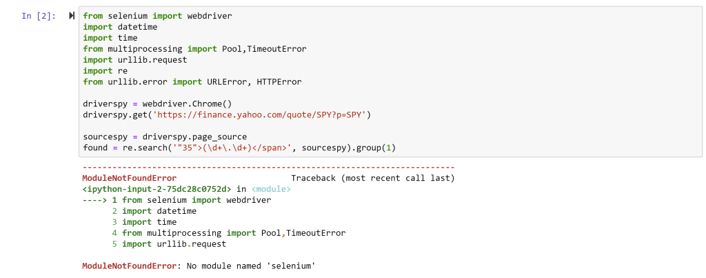
The next error you will likely receive is:

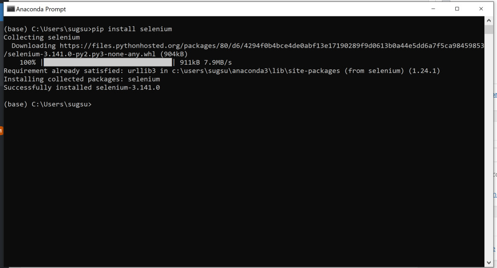
This simply says you need a package (or module) called selenium installed. On a Windows machine, this is done by opening the Anaconda Prompt (Start->Anacoda3->Anaconda Prompt) and typing in the following: pip install selenium <enter>
this should be followed by an installation taking place and some text indicating success. Something that looks like this.

If you use a Mac, you can do the same thing by opening up a terminal window and typing in the same thing.
The next error you might receive is one involving chromedriver. If might say Chromedriver is not in PATH or perhaps Chromedriver is not compatible with your version of chrome. On a PC, the first error is fixed by putting a copy of chromedriver.exe (not the zip file, and not a shortcut) in the same folder as your Python notebook. If you don’t know where your Python notebooks are in your directory structure, you can search for ipynb files in your computer. Jupyter notebook files have the extension *.ipynb so thye should be quite easy to find.
On a Mac the first error is fixed by adding the folder with Chromedriver to the system PATH (see instructions here and follow the 3rd set of instructions, adding a directory to PATH for all users, forever) . For more information on what PATH is, check out the delightful wiki on the subject.
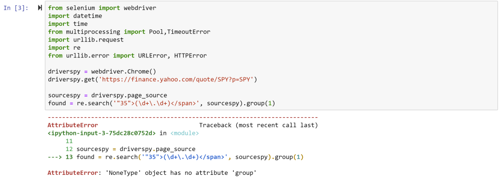
Finally, the last error you will likely get will be:

This is a cryptic error and simply means that it could not find the snippet of text the re.search command was looking for. That’s because Yahoo often changes the source code and the tag number changes from 35 to something else. AS of the time of writing ,it is 52. With that final fix, the code should be able to run.

Notice the last line I added: print(found) – without this line, the code would run, but would not do anything. The final line generates feedback to indicate success! The price of SPY at the time of running was $299.35.
So… what can we do with this? Well, we can write a small loop to get the price of SPY every few minutes. More on that in a bit….
