One of the ways I motivate using Python (over Excel) for analysis in my quantitative investing class is through simulations. Any time it is difficult to find a closed form solution, simulation is useful. Nonlinearities, such as those in hedge fund compensation contracts, are an ideal example. Is a 2/20 (referring to 2% management fee, 20% incentive fee) contract “better” than a 1.5/30 contract? Or is a 2/20 with high water mark (HWM) better than a 1.5/15 without a HWM? These questions cannot be easily answered with closed form solutions, especially if we consider some dynamics in terms of investor withdrawal, or in the fund manager’s choice of investment technology. The only way to reasonably tackle these is to simulate a bunch of outcomes and see what happens in those outcomes, to generate expected returns for the investor.
This is an ideal use case for Python, with nested “for” loops over simulation runs, and multiple time periods, with optimization by both investors and fund managers coded in. In fact, one of the (sadly unpublished) papers from my dissertation was about this. In that paper I used MATLAB for the coding, but the logic would be very similar for Python.
However, a lot of my students are not familiar with coding and as an alternative, I cover a way to use Excel to do similar analysis. The key is an off book use of the Data Table function. Data Tables are generally used for sensitivity analysis – seeing how output cells change with different input cell values.
Data tables can also be used to run simulations in Excel – for example, below is a spreadsheet that computes to the evolution of a hedge fund that starts with $100, uses a normal return technology with mean annual returns of 8% and std dev of 20%, and charged 1.5% management fee and 20% incentive fee. In the base run, this 100 dollars evolves to 120.07 at the end of 5 years. The formulae for the various computed cells are shown as well.
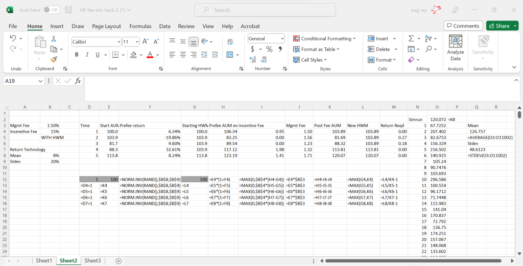
In columns N and O, we have a data table, with the first column being the run number – we are doing 10,000 runs, so while the screen shot only shows runs 1-22, there are 9,978 rows below. Unlike traditional sensitivity analysis data tables, here, we simply have the table set to input the values in column N (the sim run column) into an empty cell (for example $F$19)
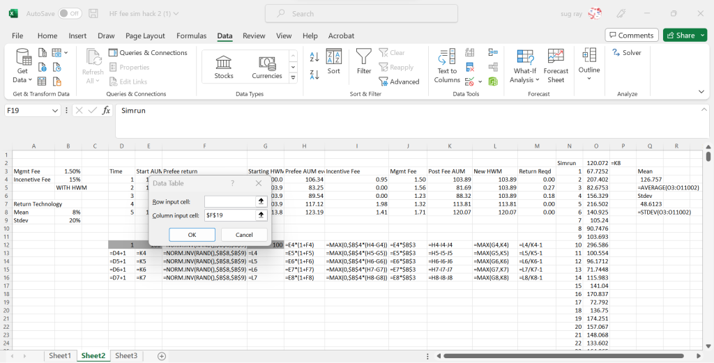
So, Excel will put 1 in F19, then record the Post Fee AUM value at the of 5 years in cell O4, then it will put 2 in F19, which will re-run all the random numbers, and put the new 5 year post fee AUM number in cell O5, and so on. At the end of this, we will get 10,000 different values of the AUM at the end of 5 years, and we can use those values to get the expected return of the fund (cell Q4). We can also get other moments, or generate VaR and CVaR type measures with these data.
It’s clunky, but it gets the job done.