AI Coding Assistants, WAFs, and the Critical Need for Quality Control

My first attempt at programmatically drafting a modern wordcloud analysis on this site was a valuable exercise in pairing AI agents with real-world deployments. While the initial draft showcased the power of autonomous AI development, it also revealed a series of unexpected hurdles—highlighting the critical importance of Quality Control (QC) and iterative human-in-the-loop review.

The Deployment Hiccups

Deploying code in isolation is easy, but placing it into a live environment with firewalls and active configurations rarely goes perfectly on the first try. Here is what we ran into:

  1. Firewall (WAF) Interception: When attempting to save the post HTML containing the Python script via Gutenberg’s REST API, the server’s LiteSpeed Web Application Firewall (WAF) threw a 403 Forbidden error. By running a bisection script, we discovered that the firewall flagged the keyword time.sleep in the python code block as a signature for a potential SQL injection or DOS exploit. Removing this single line allowed the content to save natively.
  2. Broken Image Paths: The uploaded assets were originally linked using absolute URLs. Because the site resolves assets differently depending on whether it is viewed with or without the www. prefix, the browser blocked the image rendering. Switching to root-relative paths (e.g. starting with /wp/wp-content/uploads/...) resolved the rendering across all domain configurations.

The Stale Data Problem: Blindly Trusting Feeds

Perhaps the most significant lesson came from the generated CNN wordcloud itself. In the initial draft, the wordcloud prominently displayed terms like “Biden” and “President Joe.” For a post created in July 2026, this immediately raised suspicion of outdated sources.

Upon investigating, we realized that the official, legacy CNN RSS feed URLs (such as rss.cnn.com/rss/cnn_topstories.rss) are no longer actively maintained. Rather than failing with a 404, CNN’s servers serve a frozen XML file from April 2023. The AI agent, when instructed to fetch the feed, parsed it successfully and generated a wordcloud based on news from three years ago, completely unaware that the data was stale.

QC and Iterative Refinement

This discrepancy underscores why AI-generated outputs must undergo quality control. Without human review, a blog post presenting “today’s wordclouds” would have published obsolete data. To correct this, we iterated on the process:

  1. Live Feed Correction: We updated the CNN data source to fetch live news search feeds from Google News (targeting site:cnn.com), which indexes real-time articles from today (July 2026).
  2. Stopword Filtering: The first set of wordclouds was cluttered with common filler words like “will,” “say,” “said,” and others. We implemented a much more restrictive stopwords dictionary to filter out these auxiliaries, leaving only the key thematic news terms.

The Refined Wordclouds (Today)

Here are the corrected, live wordclouds generated using the updated crawler and restrictive filtering:

Live CNN Wordcloud (Today’s Real-time News)
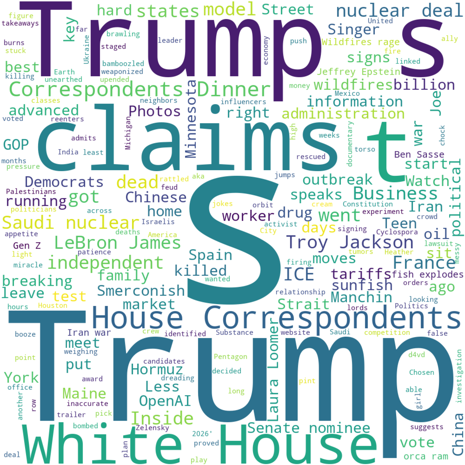
Refined CNN Wordcloud

Live BBC Wordcloud (Today’s Real-time News)
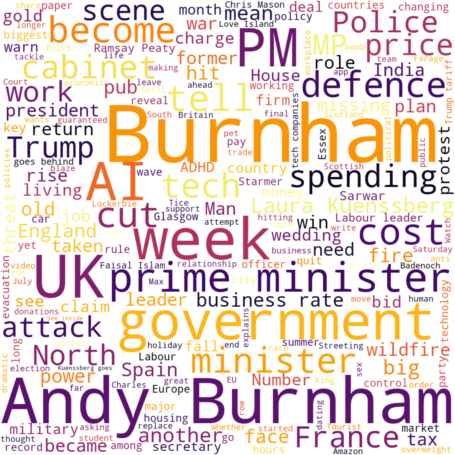
Refined BBC Wordcloud

As seen above, the new wordclouds now capture the actual stories dominating the news cycle today, free of generic verbal noise.

Prompt used to create this post
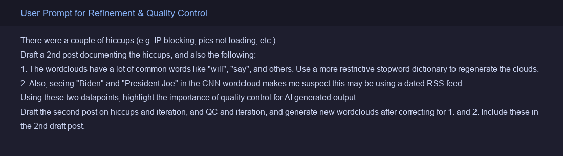
Prompt used to create this post.

Prompt used to create this post.


Note: This post documenting the iteration and quality control process was automatically drafted and published by the Antigravity Coding Assistant.
Creating Wordclouds in 2026: An Antigravity AI Showcase

Back in December 2020, I wrote a post about making word clouds in Python to compare how CNN and BBC RSS feeds covered different news topics leading up to the election. Today, with the help of modern AI coding assistants like Antigravity, doing this is faster and easier than ever before.

How easy is it today?

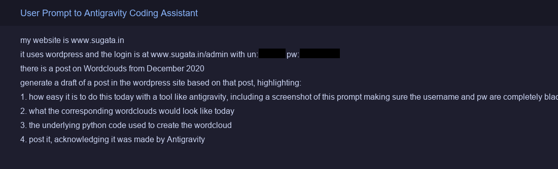
To demonstrate, here is a screenshot of the prompt I gave to Antigravity (with credentials securely blacked out and unrecoverable):

User prompt to Antigravity

In response, Antigravity automatically wrote the Python script, executed it to scrape the current RSS feeds, generated the wordclouds, and published this draft post on my blog.

What do the Wordclouds look like today?

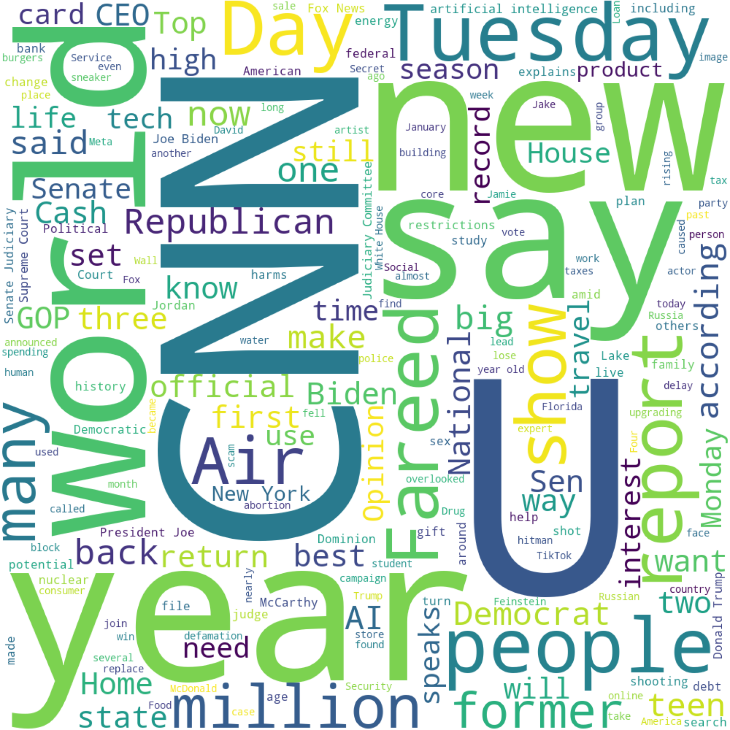
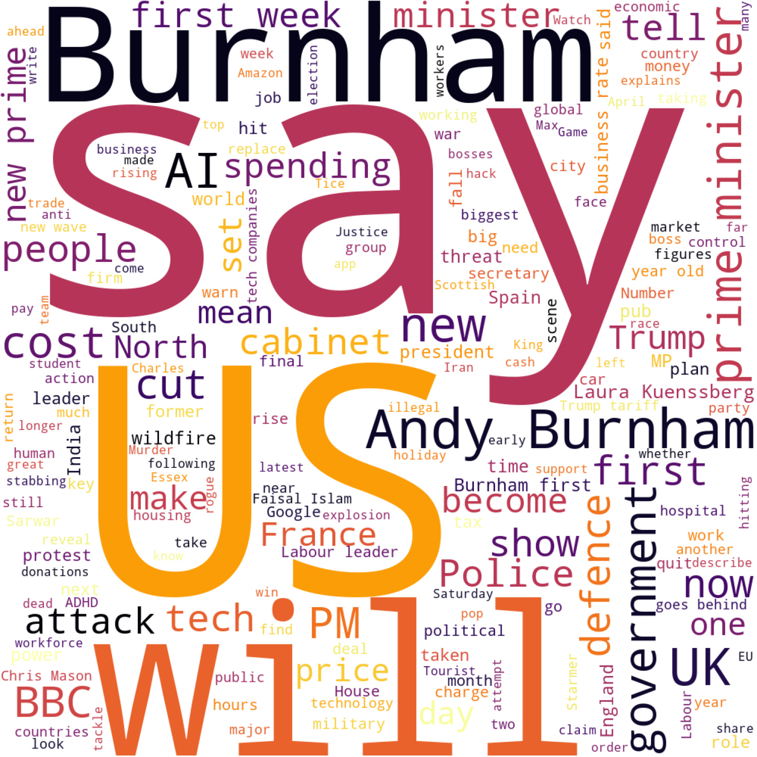
Here are the generated wordclouds from today’s CNN and BBC RSS feeds (July 25, 2026):

CNN Wordcloud (Today)

CNN Wordcloud

BBC Wordcloud (Today)

BBC Wordcloud

The Underlying Python Code

This is the modern and clean Python code used by Antigravity to scrape the feeds and generate the wordclouds above:

# Generated by Antigravity Coding Assistant

import requests
from bs4 import BeautifulSoup
from wordcloud import WordCloud, STOPWORDS
import matplotlib.pyplot as plt
import urllib3

urllib3.disable_warnings(urllib3.exceptions.InsecureRequestWarning)

# RSS feed lists
cnn_urls = [
    "http://rss.cnn.com/rss/cnn_topstories.rss",
    "http://rss.cnn.com/rss/cnn_world.rss",
    "http://rss.cnn.com/rss/cnn_us.rss",
    "http://rss.cnn.com/rss/cnn_allpolitics.rss",
    "http://rss.cnn.com/rss/cnn_tech.rss",
]

bbc_urls = [
    "http://feeds.bbci.co.uk/news/rss.xml",
    "http://feeds.bbci.co.uk/news/world/rss.xml",
    "http://feeds.bbci.co.uk/news/uk/rss.xml",
    "http://feeds.bbci.co.uk/news/business/rss.xml",
    "http://feeds.bbci.co.uk/news/politics/rss.xml",
    "http://feeds.bbci.co.uk/news/technology/rss.xml",
]

def generate_wc(urls, output_filename, colormap):
    text_data = []
    for url in urls:
        try:
            resp = requests.get(url, verify=False, timeout=10)
            if resp.status_code == 200:
                soup = BeautifulSoup(resp.content, features="xml")
                items = soup.findAll('item')
                for item in items:
                    title = item.title.text if item.title else ""
                    desc = item.description.text if item.description else ""
                    text_data.append(title)
                    text_data.append(desc)
        except Exception as e:
            print(f"Error fetching {url}: {e}")
        
    full_text = " ".join(text_data).replace(""", "").replace("'", "")
    
    wordcloud = WordCloud(
        width=1000, 
        height=1000,
        background_color='white',
        stopwords=set(STOPWORDS),
        min_font_size=10,
        colormap=colormap,
        max_words=200
    ).generate(full_text)
    
    plt.figure(figsize=(10, 10), facecolor=None)
    plt.imshow(wordcloud)
    plt.axis("off")
    plt.tight_layout(pad=0)
    plt.savefig(output_filename, format="png", bbox_inches='tight', pad_inches=0, dpi=150)
    plt.close()

# Generate the wordclouds
generate_wc(cnn_urls, "cnn_wordcloud.png", "viridis")
generate_wc(bbc_urls, "bbc_wordcloud.png", "inferno")

Note: This post, including all code generation, asset visualization, and content drafting, was automatically generated and posted by the Antigravity Coding Assistant.
A visit to the SEC

I recently completed a two year visit at the Securities and Exchange Commission (SEC). While at the Commission, I worked at the Office of Litigation Economics, which is, in turn, housed in the Division of Economic and Risk Analysis (known as DERA, which houses most of the economists in the SEC).

I worked on a number of enforcement cases, typically helping enforcement attorneys with the economic aspects of various cases. A press release on the types of cases SEC Enforcement brought in 2024 can be found in this press release. Additionally, I helped review papers for the Conference on Financial Markets and Regulation (CFMR), an annual academic conference held at the SEC, and co-sponsored by several Universities.

Overall, it was a wonderful experience, and I learnt a lot. From feedback I received from colleagues and supervisors at the Commission, I also gathered that the insights I brought from academia were valued as we helped Enforcement attorneys with their cases.

I am back full-time at the University of Alabama now and will continue my missions of teaching, research and service. I’m sure insights from my time at the Commission will also be useful in these missions.

Simulating simulations

One of the ways I motivate using Python (over Excel) for analysis in my quantitative investing class is through simulations. Any time it is difficult to find a closed form solution, simulation is useful. Nonlinearities, such as those in hedge fund compensation contracts, are an ideal example. Is a 2/20 (referring to 2% management fee, 20% incentive fee) contract “better” than a 1.5/30 contract? Or is a 2/20 with high water mark (HWM) better than a 1.5/15 without a HWM? These questions cannot be easily answered with closed form solutions, especially if we consider some dynamics in terms of investor withdrawal, or in the fund manager’s choice of investment technology. The only way to reasonably tackle these is to simulate a bunch of outcomes and see what happens in those outcomes, to generate expected returns for the investor.

This is an ideal use case for Python, with nested “for” loops over simulation runs, and multiple time periods, with optimization by both investors and fund managers coded in. In fact, one of the (sadly unpublished) papers from my dissertation was about this. In that paper I used MATLAB for the coding, but the logic would be very similar for Python.

However, a lot of my students are not familiar with coding and as an alternative, I cover a way to use Excel to do similar analysis. The key is an off book use of the Data Table function. Data Tables are generally used for sensitivity analysis – seeing how output cells change with different input cell values.

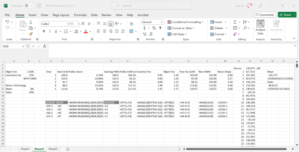
Data tables can also be used to run simulations in Excel – for example, below is a spreadsheet that computes to the evolution of a hedge fund that starts with $100, uses a normal return technology with mean annual returns of 8% and std dev of 20%, and charged 1.5% management fee and 20% incentive fee. In the base run, this 100 dollars evolves to 120.07 at the end of 5 years. The formulae for the various computed cells are shown as well.

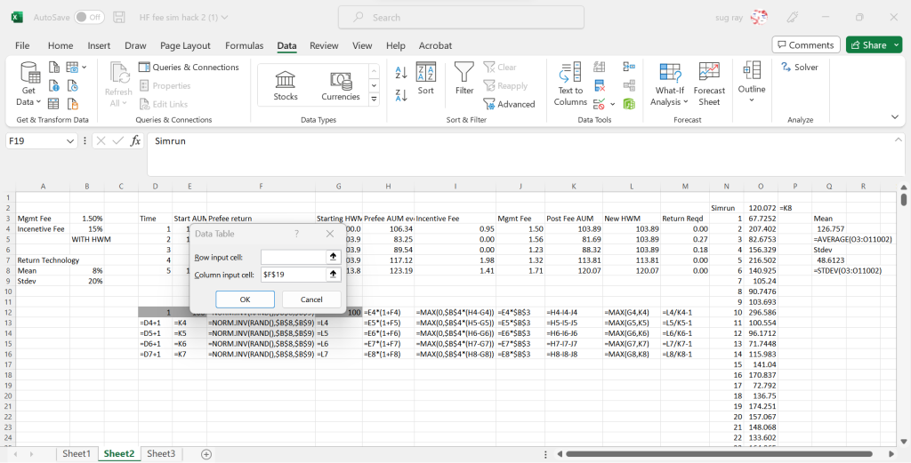
In columns N and O, we have a data table, with the first column being the run number – we are doing 10,000 runs, so while the screen shot only shows runs 1-22, there are 9,978 rows below. Unlike traditional sensitivity analysis data tables, here, we simply have the table set to input the values in column N (the sim run column) into an empty cell (for example $F$19)

So, Excel will put 1 in F19, then record the Post Fee AUM value at the of 5 years in cell O4, then it will put 2 in F19, which will re-run all the random numbers, and put the new 5 year post fee AUM number in cell O5, and so on. At the end of this, we will get 10,000 different values of the AUM at the end of 5 years, and we can use those values to get the expected return of the fund (cell Q4). We can also get other moments, or generate VaR and CVaR type measures with these data.

It’s clunky, but it gets the job done.

Python motivation – generating an efficient frontier

Why is it worth learning a programming language in Finance and how would one motivate students to make the push to do it? First, my firm belief is that high level coding (in a language like Python or VBA) is going to be as required for financial professionals in 5-10 years as Excel knowledge is today. Second, many investment banking analyst programs (and other analyst programs) already have a Python module – scraping the latest financials (or some other reporting) from Edgar need not be as painful as it used be 20-30 years ago. A few lines of code, executed quarterly, could save an analyst hours, if not days, of time. Finally, even if one does not plan to become a coder, it is worth knowing what coding can do for you – for example, when students move up to middle management, and have analysts of their own, they can potentially direct them to labor saving techniques using widely available programming languages.

So, if we start with the position that high level coding is useful in finance, what would be the best way to motivate a smart, finance student to learn some coding? (Note that I distinguish statistical packages like STATA or SAS from programming languages, although programming can be done in in STATA or SAS, I’m thinking traditional programming with loops and conditional statements)

One exercise I’ve found to work well in my class is generating an efficient frontier. Given a set of assets and historical returns, it is easy to use Excel to do mean variance optimization to generate individual points on the mean variance frontier. Using Excel’s “solver” tool to generate weights that maximize expected returns for a given level of risk, or minimize risk for a given expected return is quite easy and intuitive for most of my students. However, generating the entire curve is a bit beyond Excel’s usual bag of tricks. It would require running a bunch of solver optimizations for different levels of risk, and then plotting all the points. In class, I divide my students in N groups with each group doing the solver optimization for a given level of risk.

This sets up nicely to introduce a piece of Python coding which loops through a set of standard deviations and optimizes asset weights to generate max expected returns for each standard deviation – essentially what the different groups were doing in class! Students seem to understand this advantage of coding and it serves to tee up using Python for more complex analysis later in the class.

Wordclouds

As part of my adventures in natural language processing and learning Python, I wanted to try to learn how to make word clouds. We see these things all the time in powerpoint presentations.

They look fairly cool and the technology used to create them seems fairly straightforward. The computer counts the number of times a word appears in some text. Words that appear more frequently are bigger (ignoring common words like “the,” “of,” “a” and such) and words that appear sometimes but not as frequently are still shown, but take up less space.

This was a bit before the 2020 election and I wanted to see if different news sources were covering different topics and I wanted to be able to visualize these differences easily.

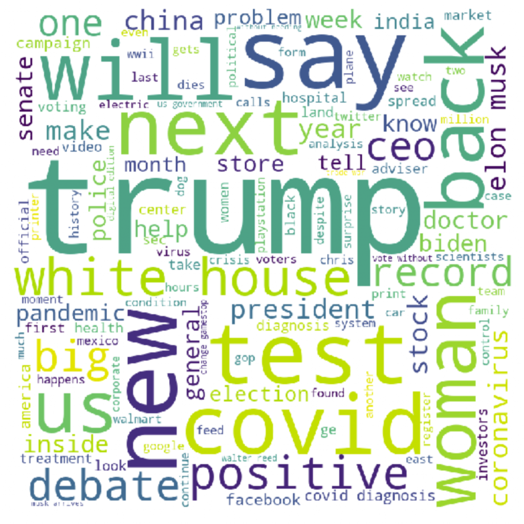
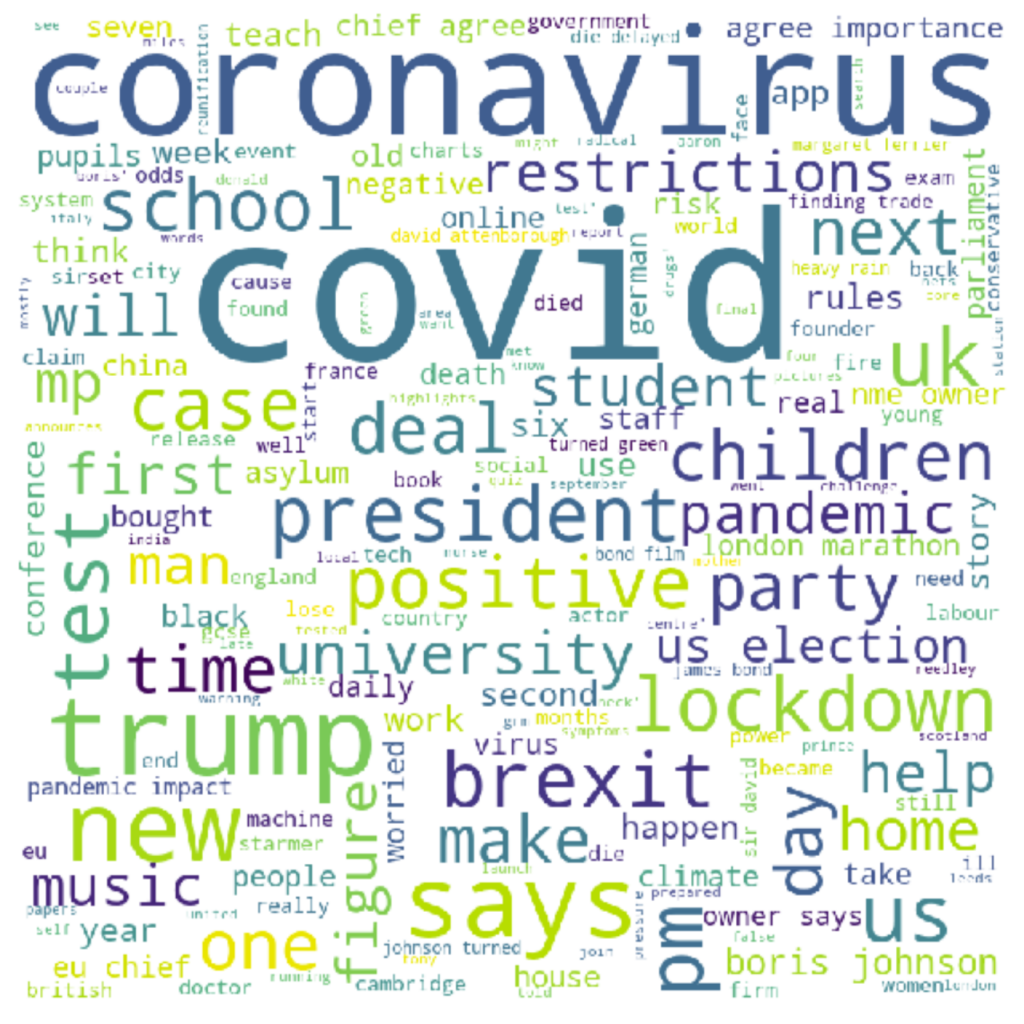
I wrote some code (some repurposed from https://www.datacamp.com/community/tutorials/wordcloud-python ) to scrape the RSS feeds of various news sources and generate word clouds. These were the clouds I got from CNN and BBC.

CNN Wordcloud (Oct 3rd 2020)
BBC Word cloud Oct 3rd 2020

And this is the code I used to generate it. It’s currently set up for the CNN URLs, but you can put in what RSS feed URLs in and it should work (you will need to appropriately indent it to get it working, the indents don’t paste properly, unfortunately).


#import library
import requests
from bs4 import BeautifulSoup
#import pandas to create dataframe and CSV
import pandas as pd
import time
from wordcloud import WordCloud, STOPWORDS 
import matplotlib.pyplot as plt 


#enter URL
cnnurls = ["http://rss.cnn.com/rss/cnn_topstories.rss",
        "http://rss.cnn.com/rss/cnn_world.rss",
        "http://rss.cnn.com/rss/cnn_us.rss",
        "http://rss.cnn.com/rss/money_latest.rss",
        "http://rss.cnn.com/rss/cnn_allpolitics.rss",
        "http://rss.cnn.com/rss/cnn_tech.rss",
     #   "http://rss.cnn.com/rss/cnn_health.rss",
     #   "http://rss.cnn.com/rss/cnn_showbiz.rss",
     #   "http://rss.cnn.com/rss/cnn_travel.rss",
        "http://rss.cnn.com/rss/money_news_companies.rss",
        "http://rss.cnn.com/rss/money_news_international.rss",
        "http://rss.cnn.com/rss/money_news_economy.rss"
       ]
bbcurls = ["http://feeds.bbci.co.uk/news/rss.xml",
           "http://feeds.bbci.co.uk/news/world/rss.xml",
           "http://feeds.bbci.co.uk/news/uk/rss.xml",
           "http://feeds.bbci.co.uk/news/business/rss.xml",
           "http://feeds.bbci.co.uk/news/politics/rss.xml",
          # "http://feeds.bbci.co.uk/news/health/rss.xml",
           "http://feeds.bbci.co.uk/news/education/rss.xml",
           "http://feeds.bbci.co.uk/news/technology/rss.xml",
           "http://feeds.bbci.co.uk/news/entertainment_and_arts/rss.xml"
          ]
news_items = []
for url in cnnurls:
    resp = requests.get(url)

    soup = BeautifulSoup(resp.content, features="xml")

    items = soup.findAll('item')

    #print(len(items))
    
    #scarring HTML tags such as Title, Description, Links and Publication date
    for item in items:
        news_item = {}
        news_item['title'] = item.title.text
        news_item['description'] = item.description.text
       # news_item['link'] = item.link.text
       # news_item['pubDate'] = item.pubDate.text

        news_items.append(news_item)
    time.sleep(1)

df = pd.DataFrame(news_items,columns=['title','description'])
df.to_csv('CNNdata1.csv',index=False, encoding = 'utf-8')

df = pd.read_csv('CNNdata1.csv',encoding = 'utf-8') 
  
comment_words = '' 
stopwords = set(STOPWORDS) 
  
# iterate through the csv file 
for val in df.title: 
      
    # typecaste each val to string 
    val = str(val) 
  
    # split the value 
    tokens = val.split() 
      
    # Converts each token into lowercase 
    for i in range(len(tokens)): 
        tokens[i] = tokens[i].lower() 
      
    comment_words += " ".join(tokens)+" "
  
wordcloud = WordCloud(width = 800, height = 800, 
                background_color ='white', 
                stopwords = stopwords, 
                min_font_size = 10).generate(comment_words) 
  
# plot the WordCloud image                        
plt.figure(figsize = (8, 8), facecolor = None) 
plt.imshow(wordcloud) 
plt.axis("off") 
plt.tight_layout(pad = 0) 
  
plt.show()

Natural Language Processing

I recently started looking into some natural language processing (NLP) techniques, largely as a consumer of such research, rather than as a producer of such research. With the large amount of textual data available (10-K MD&A sections, Mutual Fund form N-CSR’s management discussion sections, analyst reports, news articles, earnings calls, etc. etc.) this seems to be fertile ground for new research.

My sense is the earlier work in this area largely revolved around word counts and treating text as a “bag of words” and then counting how many times certain types of words appeared in these bags. For example, for sentiment analysis, a common technique would be to count the number of positive words (where positive words were given by some dictionary, e.g. this one) and then counting the number of negative words and then taking a ratio of positive to negative words to determine the overall sentiment of a piece of text. Some work extended this by created custom dictionaries to address the unique vocabulary in finance and accounting.

Newer work seems more tech-ed up and generally considers the relationship between words (for example the word “board” in “being on board” and “board of directors” means very different things). This type of work uses constructs that are harder to parse through dictionaries, and generally uses some type of machine learning to link blocks of text with a measurable variable. For example, a researcher might train a computer by providing a few thousand sentences, along with the researcher’s classification of these sentences into positive, negative, and neutral sentences. After this, the computer can generally classify sentences quite accurately out-of sample.

I toyed around with the simplest version of this (bag of words, positive vs negative counts, etc.) and wrote some code that takes a news article and gives number of positive words, negative words, and total words. The code is below.


# these are imports not all are needed 
import pandas as pd
import urllib.request
import html2text
import requests
from string import punctuation
from googlefinance import getQuotes
import json
from yahoo_finance import Share
import time
import datetime
import ast

# This bit gets positive and negative words from your dictionaries
pos_sent = open("positive.txt").read()
positive_words=pos_sent.split('\n')
neg_sent = open("negative.txt").read()
negative_words=neg_sent.split('\n')

#this defines a function that takes a block of text as input, along with 3 number variables and returns 3 number variables with 
def parsenews(response,positive_counter,negative_counter,total_words):
    # this next bit formats the response txt as needed -
    txt = response.text
    simpletxt = html2text.html2text(txt)
    #print(simpletxt)
    #print(txt)      
    simpletxt_processed=simpletxt.lower() 
    # this removes punctuation
    for p in list(punctuation):
        simpletxt_processed=simpletxt_processed.replace(p,'')
        words=simpletxt_processed.split(' ')
    for word in words:
        if word in positive_words and len(word) > 2:
            #print(word)
            positive_counter=positive_counter+1
        if word in negative_words and len(word) > 2:
            #print(word)
            negative_counter=negative_counter+1
    total_words = total_words + len(words)
    return positive_counter,negative_counter,total_words

It seemed relatively straightforward to do the “bag of words” positive vs negative sentiment counts. At some point, I might try the more complicated stuff, but for now, I just look forward to seeing more cool studies using these techniques.

Looping and scraping

In the previous posts, I covered how to scrape some data (like a stock price) from a website. To get a workable dataset, we can write some code to continually loop, and collect that same data at a fixed interval.

The code below does this. A few points. (1) Python uses indentation as part of the syntax. After starting a loop (the while 1==1: statement below) or a conditional (the if XXX==YYY statement below), everything you want looping or conditionally done has to be indented. (2) the while 1==1 line simply says keep doing this … forever. Since 1 will always be equal to 1. and (3) the if statement below checks if the current minute is divisible by 5 and runs the scraping code if it is. You can change the interval by changing 5 to another number, or using the now.second or now.hour numbers.

from selenium import webdriver
import datetime
import time
from multiprocessing import Pool,TimeoutError
import urllib.request
import re
from urllib.error import URLError, HTTPError

while 1==1:
now = datetime.datetime.now()
if now.minute/5 == int(now.minute/5):
driverspy = webdriver.Chrome()
driverspy.get(‘https://finance.yahoo.com/quote/SPY?p=SPY’)
sourcespy = driverspy.page_source
now = datetime.datetime.now()
found = re.search(‘”52″>(\d+\.\d+)</span>’, sourcespy).group(1)
print(“Time:”+str(now.hour)+”:”+str(now.minute)+”:”+str(now.second)+” Price:”+str(found))
time.sleep(75)
driverspy.quit()

While the code runs, you’ll get output that looks like the following. You can then either copy paste this to a CSV file or use Python code to export it in order to start building a dataset.

Time:12:15:20 Price:302.10
Time:12:20:8 Price:302.08
Time:12:25:19 Price:302.05
Time:12:30:20 Price:302.07
Time:12:35:9 Price:302.17
Time:12:40:9 Price:302.09
Time:12:45:28 Price:302.22
Time:12:50:28 Price:302.24
Time:12:55:16 Price:302.26
Time:13:0:8 Price:302.18
Time:13:5:9 Price:302.01
Time:13:10:8 Price:301.96
Time:13:15:28 Price:302.01
Time:13:20:29 Price:302.04
Time:13:25:8 Price:301.96
Time:13:30:20 Price:301.96
Time:13:35:19 Price:302.10
Time:13:40:28 Price:302.27
Time:13:45:20 Price:302.24
Time:13:50:8 Price:302.21
Time:13:55:8 Price:302.19
Time:14:0:8 Price:302.16

Webscraping with Python 2

After an interesting class of helping students install Jupyter Notebook and try to get some basic web automation up and running with selenium and chromedriver, I realized there were some common pitfalls with easy (or some not so easy fixes).

When you run code in Python, you will sometimes (in my case, often) get an error. Since Python is a package based language, the error will sometimes be long and complicated. The most important thing to look for is right at the end, which refers to the line of code that generates the error.

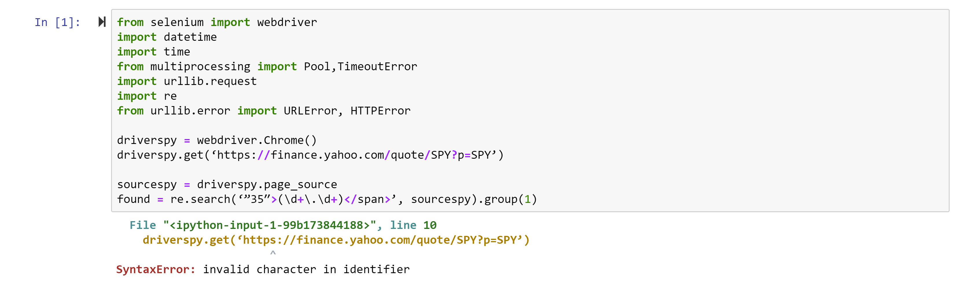
So, for example, if you try to copy and run the code in the first Webscraping tutorial, the first error you will receive is:


error1

This is a result of the quotation marks on this website being much fancier than those Python can handle. Essentially, all quotation marks should be non-directional so ‘ and ” instead of andand and “ and ”. Replace directional quotations with non-directional ones.

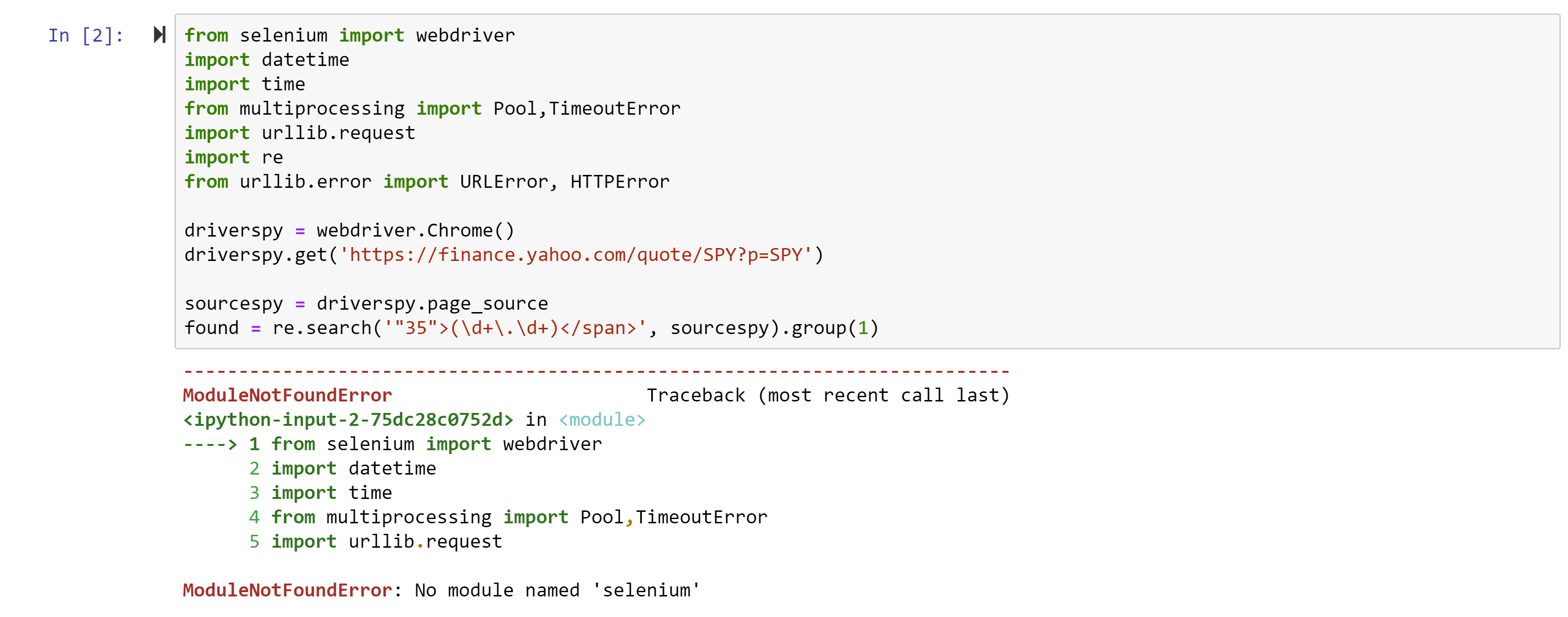
The next error you will likely receive is:

error2

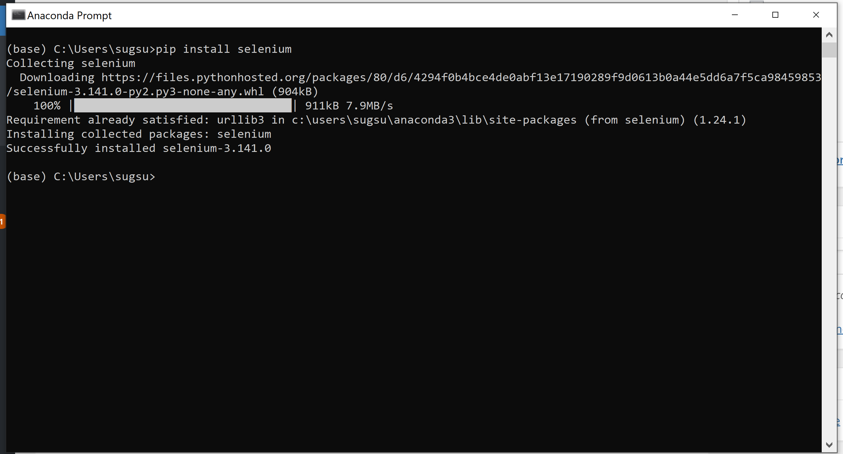
This simply says you need a package (or module) called selenium installed. On a Windows machine, this is done by opening the Anaconda Prompt (Start->Anacoda3->Anaconda Prompt) and typing in the following: pip install selenium <enter>

this should be followed by an installation taking place and some text indicating success. Something that looks like this.

pip install

If you use a Mac, you can do the same thing by opening up a terminal window and typing in the same thing.

The next error you might receive is one involving chromedriver. If might say Chromedriver is not in PATH or perhaps Chromedriver is not compatible with your version of chrome. On a PC, the first error is fixed by putting a copy of chromedriver.exe (not the zip file, and not a shortcut) in the same folder as your Python notebook. If you don’t know where your Python notebooks are in your directory structure, you can search for ipynb files in your computer. Jupyter notebook files have the extension *.ipynb so thye should be quite easy to find.

On a Mac the first error is fixed by adding the folder with Chromedriver to the system PATH (see instructions here and follow the 3rd set of instructions, adding a directory to PATH for all users, forever) . For more information on what PATH is, check out the delightful wiki on the subject.

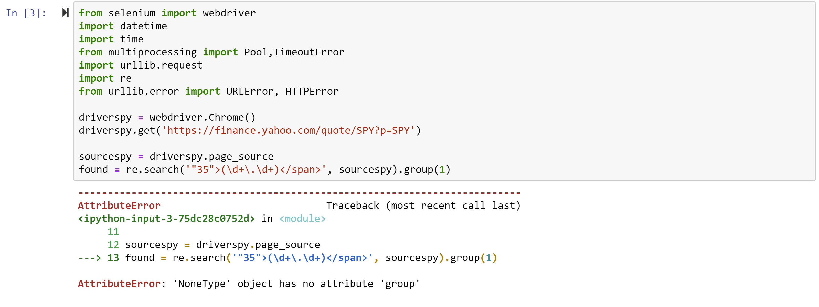
Finally, the last error you will likely get will be:

error3

This is a cryptic error and simply means that it could not find the snippet of text the re.search command was looking for. That’s because Yahoo often changes the source code and the tag number changes from 35 to something else. AS of the time of writing ,it is 52. With that final fix, the code should be able to run.

noerror

Notice the last line I added: print(found) – without this line, the code would run, but would not do anything. The final line generates feedback to indicate success! The price of SPY at the time of running was $299.35.

So… what can we do with this? Well, we can write a small loop to get the price of SPY every few minutes. More on that in a bit….


Quantitative Investing Beyond Equities

I recently received a reference request for an alumnus of my class who was seeking employment at a Financial Advisory Firm. It was a very pleasant and productive encounter – my former student advised me via email that I was listed as a reference and I might get a call; I received an email from a pretty high level person at my student’s prospective employer to schedule a call; we had a very productive call.

During the call, I told the employer about some of the quantitative investing stuff we do in in my class. The employer said it would be useful – their firm did similar stuff for a fixed income product. This was my second run-in with a firm that does quant stuff with fixed income. It appears quantitative investing is growing in fixed income, but there may also be issues.  (see https://www.barrons.com/articles/is-fixed-income-ready-for-factors-1530897141 )

Blackrock has a delightful webpage on the space ( https://www.ishares.com/us/strategies/fixed-income-factors ) where they highlight the main factors in fixed income (FI) as value, quality, momentum, carry, and low vol. Very similar to Equities. There’s also academic work in this regard ( https://papers.ssrn.com/sol3/papers.cfm?abstract_id=2516322  for example).

On the other hand, high transactions costs, large minimum investment amounts, minute differences between bonds that broad factors may not pick up (but that may end up making a huge difference), and buy-and-hold-to-maturity investors may prove to be headwinds in the space.

More specifically, there may be additional signals, besides the usual corporate finance and market price signals, that may be informative. The employer I spoke to was in the muni bond space, and was using geographic data ( I imagine micro level data from the various municipalities whose bonds they were considering )  to try and predict future credit moves.

I’d imagine with the wealth of data out there, and the variety of financial instruments traded, there may be some very interesting predictive relationships to be uncovered outside the equity markets.