I recently completed a two year visit at the Securities and Exchange Commission (SEC). While at the Commission, I worked at the Office of Litigation Economics, which is, in turn, housed in the Division of Economic and Risk Analysis (known as DERA, which houses most of the economists in the SEC).
I worked on a number of enforcement cases, typically helping enforcement attorneys with the economic aspects of various cases. A press release on the types of cases SEC Enforcement brought in 2024 can be found in this press release. Additionally, I helped review papers for the Conference on Financial Markets and Regulation (CFMR), an annual academic conference held at the SEC, and co-sponsored by several Universities.
Overall, it was a wonderful experience, and I learnt a lot. From feedback I received from colleagues and supervisors at the Commission, I also gathered that the insights I brought from academia were valued as we helped Enforcement attorneys with their cases.
I am back full-time at the University of Alabama now and will continue my missions of teaching, research and service. I’m sure insights from my time at the Commission will also be useful in these missions.
One of the ways I motivate using Python (over Excel) for analysis in my quantitative investing class is through simulations. Any time it is difficult to find a closed form solution, simulation is useful. Nonlinearities, such as those in hedge fund compensation contracts, are an ideal example. Is a 2/20 (referring to 2% management fee, 20% incentive fee) contract “better” than a 1.5/30 contract? Or is a 2/20 with high water mark (HWM) better than a 1.5/15 without a HWM? These questions cannot be easily answered with closed form solutions, especially if we consider some dynamics in terms of investor withdrawal, or in the fund manager’s choice of investment technology. The only way to reasonably tackle these is to simulate a bunch of outcomes and see what happens in those outcomes, to generate expected returns for the investor.
This is an ideal use case for Python, with nested “for” loops over simulation runs, and multiple time periods, with optimization by both investors and fund managers coded in. In fact, one of the (sadly unpublished) papers from my dissertation was about this. In that paper I used MATLAB for the coding, but the logic would be very similar for Python.
However, a lot of my students are not familiar with coding and as an alternative, I cover a way to use Excel to do similar analysis. The key is an off book use of the Data Table function. Data Tables are generally used for sensitivity analysis – seeing how output cells change with different input cell values.
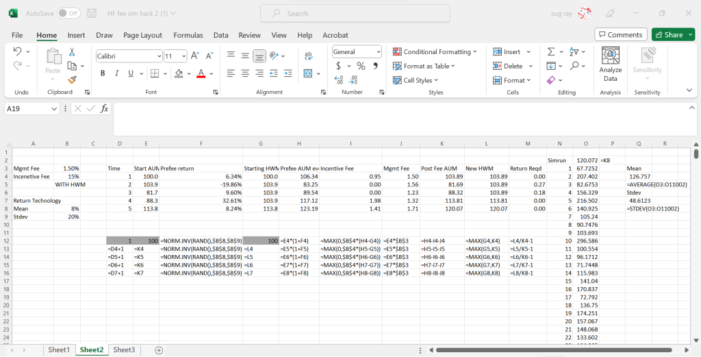
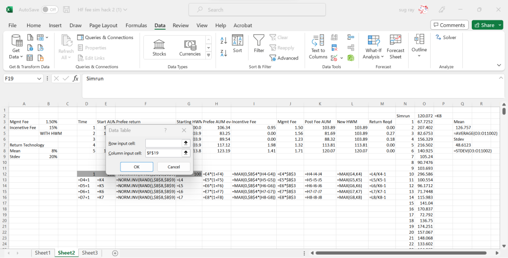
Data tables can also be used to run simulations in Excel – for example, below is a spreadsheet that computes to the evolution of a hedge fund that starts with $100, uses a normal return technology with mean annual returns of 8% and std dev of 20%, and charged 1.5% management fee and 20% incentive fee. In the base run, this 100 dollars evolves to 120.07 at the end of 5 years. The formulae for the various computed cells are shown as well.
In columns N and O, we have a data table, with the first column being the run number – we are doing 10,000 runs, so while the screen shot only shows runs 1-22, there are 9,978 rows below. Unlike traditional sensitivity analysis data tables, here, we simply have the table set to input the values in column N (the sim run column) into an empty cell (for example $F$19)
So, Excel will put 1 in F19, then record the Post Fee AUM value at the of 5 years in cell O4, then it will put 2 in F19, which will re-run all the random numbers, and put the new 5 year post fee AUM number in cell O5, and so on. At the end of this, we will get 10,000 different values of the AUM at the end of 5 years, and we can use those values to get the expected return of the fund (cell Q4). We can also get other moments, or generate VaR and CVaR type measures with these data.
I recently started looking into some natural language processing (NLP) techniques, largely as a consumer of such research, rather than as a producer of such research. With the large amount of textual data available (10-K MD&A sections, Mutual Fund form N-CSR’s management discussion sections, analyst reports, news articles, earnings calls, etc. etc.) this seems to be fertile ground for new research.
My sense is the earlier work in this area largely revolved around word counts and treating text as a “bag of words” and then counting how many times certain types of words appeared in these bags. For example, for sentiment analysis, a common technique would be to count the number of positive words (where positive words were given by some dictionary, e.g. this one) and then counting the number of negative words and then taking a ratio of positive to negative words to determine the overall sentiment of a piece of text. Some work extended this by created custom dictionaries to address the unique vocabulary in finance and accounting.
Newer work seems more tech-ed up and generally considers the relationship between words (for example the word “board” in “being on board” and “board of directors” means very different things). This type of work uses constructs that are harder to parse through dictionaries, and generally uses some type of machine learning to link blocks of text with a measurable variable. For example, a researcher might train a computer by providing a few thousand sentences, along with the researcher’s classification of these sentences into positive, negative, and neutral sentences. After this, the computer can generally classify sentences quite accurately out-of sample.
I toyed around with the simplest version of this (bag of words, positive vs negative counts, etc.) and wrote some code that takes a news article and gives number of positive words, negative words, and total words. The code is below.
# these are imports not all are needed
import pandas as pd
import urllib.request
import html2text
import requests
from string import punctuation
from googlefinance import getQuotes
import json
from yahoo_finance import Share
import time
import datetime
import ast

# This bit gets positive and negative words from your dictionaries
pos_sent = open("positive.txt").read()
positive_words=pos_sent.split('\n')
neg_sent = open("negative.txt").read()
negative_words=neg_sent.split('\n')

#this defines a function that takes a block of text as input, along with 3 number variables and returns 3 number variables with
def parsenews(response,positive_counter,negative_counter,total_words):
    # this next bit formats the response txt as needed -
    txt = response.text
    simpletxt = html2text.html2text(txt)
    #print(simpletxt)
    #print(txt)
    simpletxt_processed=simpletxt.lower()
    # this removes punctuation
    for p in list(punctuation):
        simpletxt_processed=simpletxt_processed.replace(p,'')
        words=simpletxt_processed.split(' ')
    for word in words:
        if word in positive_words and len(word) > 2:
            #print(word)
            positive_counter=positive_counter+1
        if word in negative_words and len(word) > 2:
            #print(word)
            negative_counter=negative_counter+1
    total_words = total_words + len(words)
    return positive_counter,negative_counter,total_words
It seemed relatively straightforward to do the “bag of words” positive vs negative sentiment counts. At some point, I might try the more complicated stuff, but for now, I just look forward to seeing more cool studies using these techniques.
One part of my academic research agenda deals with the effects of limited attention on professional investing. This paper uses marital events as a shock to attention and shows how managers behave differently when they’re getting married or divorced. We find that managers in general become less active in their trading/investing, suffer from behavioral biases more, and perform poorer.
This past semester, I moved from the Univ. of Florida to the Univ. of Alabama and prepped a couple of new classes. While not as stressful as marriage or divorce, I did devote a bit less time to my portfolio this semester … so what happened in my case?
The biggest change was (1) I rebalanced less… I probably ran my screen once or twice the entire semester to look for equities to deploy assets to. (2) I did not, even once, look for improvements to my screens or run any of my secondary screens.
The effects were not immediately felt on performance, but I suspect if I continued on this “autopilot” path, so to speak, the end result would be a less than manicured portfolio and eventually, a stale and less than robust investment screen. All in all, I feel my personal experience is consistent with what we found in the paper above.
With my recent move to the University of Alabama from the University of Florida, I starting thinking about the topic of change. In the context of quantitative investing, I started thinking about changes in basic rules that we take for given when investing quantitatively and what we can do about them.
Here’s an example – academics have long taught the CAPM, a model that predicts that companies with higher systematic risk (risk stemming from overall market conditions) should outperform companies with lower systematic risk. This makes intuitive sense… riskier companies, especially companies with higher risk exposure to overall economic conditions *should* give higher returns, on average. The empirical evidence in the 70s and 80s (in hindsight) was mixed, but in general we accepted this wisdom.
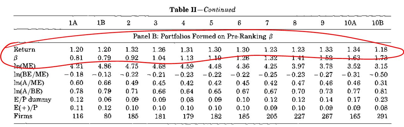
However, starting in the 1990s, we started to question this basic assumption. Fama French 1992, Table II documented this:
Companies are sorted by “pre-ranking betas” (simply the beta estimated using data from before the period we measure the returns) and the average monthly returns for the next year, by pre-beta deciles are presented. 1A and 1B are the 0-5% and 5-10% comapnies by pre-rnaking beta, 2-9 are the 2nd through 9th decile by pre-ranking beta, 10A and 10B are the 90-95% and 95-100% of firms by preranking beta.
Fama and French wrote, “the beta-sorted portfolios do not support the [CAPM]. … There is no obvious relation between beta and average returns.” [disclaimer: to my eyes, if I squint hard enough, I can sort of see a slight increase in average returns with beta, but the magnitude and monotonicity of the effect are both questionable.]
And so the decline of empirical belief in the CAPM started, and today, there is little faith that stocks with high market betas will outperform the market (although the CAPM is still widely taught). (see, for example “Is Beta Dead” from the Appendix of a popular Finance Textbook. )
In fact, the academic literature has made something of a 180 on this topic. The new hot anomaly is “low vol,” or “low beta.” This literature around this anomaly shows that the low volatility/low beta stocks actually outperform high volatility/high beta stocks and proposes several stories as to why this might be the case. If something so firmly grounded in theory can experience so complete a change, I think it’s a cautionary tale for *all* quantitative strategies … all things (including both the CAPM Beta and my time at Florida), run their course eventually.
In a new academic piece, we examine whether anomalies themselves exhibit momentum. Momentum in the context of investing refers to the idea that stocks that have done well recently continue to do well and stocks that have done poorly recently continue to do poorly. The momentum anomaly in stocks was widely publicized by Jagadeesh and Titman in their 1993 paper titled, “Returns to Buying Winners and Selling Losers: Implications for Stock Market Efficiency.”
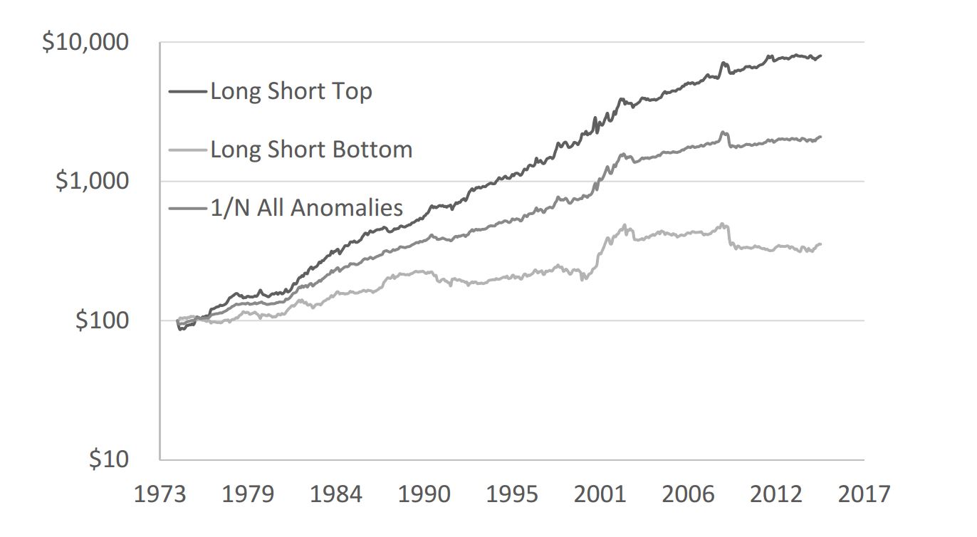
We find this same idea holds for anomalies themselves. Examining 13 anomalies, we find anomalies that have performed well recently (in the last month), continue to do well next month. Anomalies that have been performing poorly recently continue to experience poor performance going forward. A chart makes this clear:
The chart documents the evolution of $10,000 invested in one of three strategies. The top line is a strategy that invests each month in the top half of the 13 anomalies (7 since investing in 6½ anomalies is hard) being analyzed, based on the 13 anomalies’ performance in the previous month. So, for example, if the value, momentum, size, profitability, accruals, investment level, and O-score anomalies did better than the other 6 anomalies we analyzed\ last month, the strategy would equally invest in these 7 anomalies. The bottom line does the opposite, investing in the bottom 6 anomalies and the middle line equally invests in all 13 anomalies across the entire period.
From the chart, it is clear that anomalies themselves exhibit momentum and the result is robust to the usual battery of academic tests. From a practitioner’s perspective, the implication is clear: if you’re interested in smart beta type investing, pick a strategy (or strategies) that has been doing well recently. From an academic’s perspective, the more interesting question is why. If you’re interested in our take on reasons for this, you can read our paper for some reasons we think we observe this momentum across anomalies.
With the Dow and other indices at record levels, there is no shortage of pundits out there warning of an impending correction, or worse. See, for example, http://money.cnn.com/2016/04/15/investing/stock-market-donald-trump-ted-cruz/ and http://thesovereigninvestor.com/exclusives/80-stock-market-crash-to-strike-in-2016/ .
Some of the fear mongers, unfortunately, have an ulterior motive for predicting doom and gloom. A number of advisers look at such predictions as free options – if there is a crash, they can sagely point to their warnings and say, “See, I called it.” Some can even monetize their call… raising funds as investors look to re-allocate their decimated portfolios to stem the bleeding. If there is no crash, well, no one will look back and call them out on their incorrect call.
To me, the real question is whether these prognosticators have their money where their mouth is. If they think a major crash is coming, are they short? Or at least in cash? If not, I find their warnings have little credibility. They might be right, they might be wrong – either way, they’re not betting their own money on the call.
As the famous saying from Paul Samuelson goes, Economists (using technical indicators), “predicted nine of the last five recessions.” It wouldn’t surprise me if unscrupulous financial advisers and nay-saying pundits predicted ninety.
I have recently been working on an academic paper on using multiple factors to invest. This is a marked departure from most of my other academic work (which generally involves hedge fund data). This research is also directly relevant to my investing work. While the research itself is still ongoing and I am not ready to share the conclusions, I had a couple of insights on how difficult it is to combine factors that I’d share.
The technique I’ve been using to combine factors is looking for intersections – I believe value stocks outperform growth stocks and past winners outperform losers. I want to buy stocks that are both value stocks AND past winners. (Incidentally, there is a rigorous academic paper arguing for this exact factor combination by the managers of one of the most successful quantitative investing shops).
This works well… to an extent. The more factors you add, the fewer stocks will get through. As an example, if you wanted the top 10% of stocks by value (say P/E ratios) and the top 10% of stocks by past returns, and the two were uncorrelated, your filter would return about 1% of stocks in the universe. Adding a 3rd uncorrelated factor, say size (small cap firms generally outperform larger ones), would reduce the filtered stocks even further to about 0.1% of stocks in the universe.
Beyond 3 factors, it is impossible to use intersections to combine factors. The resulting sample size is simply too small. One could (and I have) relaxed the constraints on each individual constraint, and in that manner blend more factors, but this feels artificial and might even be to the detriment of the screen.
To use a sports analogy (and since the NBA championships are on), I could ask for the top 10% of 3 point shooters and top 10% of overall point scorers and I’d probably get Stephen Curry and a few others. If I then add top 10% of assists to my criteria, I probably won’t have a single player in the league fitting the bill. IF I then relax my criteria to be the top 30% of 3 point shooters, overall point scorers and assists, I’d probably get players in there again, but it’s unclear I’d like them over my original 2 factor criteria that returned Curry and co.
The January Effect refers to the observation that stock returns appear much higher in January than other months. There’s a beautiful wiki on the effect ( https://en.wikipedia.org/wiki/January_effect ) so I won’t go into much detail on it, except to say that:
1. The first thing that came to my mind regarding this effect is taxes – people sell in December to harvest tax losses/gains and then rebuy in January
2. From my understanding, this effect may no longer exist – papers come out both ways on this with recent data.
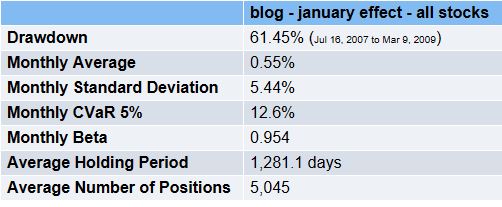
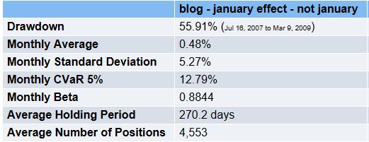
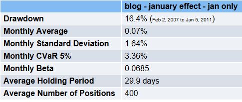
3. Here’s what Equities Lab has to say about the issue.I ran three backtests – all used data from Jan 1 2000 to today, had a monthly rebalance over all stocks (including illiquid small stocks) – the first does all months, the second does all months except January and the third does January only.
To compare the three, we can normalize everything to 12 month returns –
All months annual returns = 1.0055^12 –> 6.8%
Non January returns = (1.0048^(12/11))^12 –> 6.5%
January only returns = (1.0007^(12/1))^12 –> 10.6%
In light of this evidence, I think there’s a case to be made that some version of the January Effect still exists.